VII MUNRO’S FINITE ELEMENT METHOD IN ELECTRON OPTICS

 

Extracts from Cambridge University Ph.D. Dissertation by E Munro

Compiled and Edited by K. C. A. Smith

 

I. INTRODUCTION

 

The introduction of the finite-element method by Eric Munro (Munro 1970) opened a new era in electron optics. Previous methods of dealing with the analysis and design of electron lenses, such as finite difference or analogue resistance network techniques, were totally inadequate for lenses with complicated pole-piece shapes or for saturated magnetic lenses; Munro’s methods offered comparative freedom to the designer of complex electron optical systems, including ones combining electrostatic and magnetic elements. The methods devised by Munro represent perhaps the most significant contribution to electron optics in the period under review.

I chapter 5.3 of Volume 133 (page 438) Munro describes how Ron Ferrari, his PhD supervisor, suggested that he should attend a lecture given by a visiting lecturer to the CUED, Professor Zienkiewicz of the University of Wales at Swansea. The lecture concerned the application of finite elements in soil mechanics. During the lecture it suddenly struck Munro that the non-linear stress-strain curves relating to mud that the lecturer was presenting looked exactly like the non-linear magnetization curves for magnetic materials, and that the same mathematical formalism used to predict the behaviour of mud could almost certainly be used for saturated electron lens design.

Eric Munro also describes in his chapter in Volume 133 how Charles Oatley acted as his mentor throughout his research studies; it was fitting therefore that one of the first applications of the finite element method in electron optics was for the design of a new lens for an experimental SEM that Oatley was constructing at the time. An indication of the nature and scope of Munro’s work is to be found in the introductory chapter to his PhD dissertation (Munro 1971), reproduced in full below.

 

A. Computer-aided Design Methods in Electron Optics: Introduction

(Extracts from PhD Dissertation, Munro 1971)

 

This dissertation describes new computer-aided-design methods for use in electron optics. The methods have been used to design better lenses and detectors for electron microscopes. New lenses have been designed with very low aberration coefficients; these provide higher resolution and easier specimen manipulation in transmission electron microscopes, and allow a reduction in image recording time in scanning electron microscopes. New secondary electron detectors for scanning electron microscopes have been designed with very high contrast coefficients; these can provide enhanced contrast from specimens in the scanning electron microscope.

In Chapter 2, previous methods for determining potential distributions in electron lenses are reviewed, and the limitations of such methods are pointed out. It is shown that all these limitations can be overcome by using the 'finite element method', a numerical technique which has not been used previously in electron optics. The finite element method offers the following advantages over all previous methods:

Lenses with pole-pieces of any shape can be analysed.

The finite permeability of the pole-pieces can be taken into account.

The flux distribution throughout the magnetic circuit, including the coil windings, can be computed.

Magnetic lenses can be analysed under saturation conditions, taking the non-linearity of the magnetisation characteristic into account.

Lenses with superconducting shielding cylinders, and iron-free mini-lenses, can be dealt with.

Chapters 3 – 5 describe how the finite element method has been used to compute potential distributions in electron lenses Chapter 3 explains how the method is used to compute the scalar potential distribution in the pole-piece region of any lens. Chapter 4 shows how the method is used to compute the vector potential distribution throughout the magnetic circuit of a lens. Chapter 5 describes the extension of the method to deal with saturated magnetic lenses.

The accuracy of the computer programs has been checked using analytic mathematical tests and comparisons with the results of previous authors (Chapter 6). The computed field distribution in a saturated magnetic lens has been compared with experimental measurements (Chapter 7). These tests have shown that the computed field distributions are accurate to within l% in the case of unsaturated lenses, and to within 5% in the case of saturated lenses.

After the finite element programs have been used to compute the axial field distribution of any-lens, its optical properties can be computed using the program described in Chapter 8. Tests have shown that the computed optical properties are within 1% of the true values.

The new programs have been used to compute the properties of a wide range of electron lenses. Many new lens designs are presented (Chapters 9–13), which illustrate the versatility and wide range of application of the programs.

Chapter 9 presents a new design of probe-forming lens with a spherical aberration coefficient 2.5 times smaller than previously published values. This new lens enables the image recording time in the scanning electron microscope to be reduced by a factor of 1.8, for a given resolution and signal-to-noise ratio. The new lens has been built, and its aberration coefficients have been measured experimentally. The agreement between measured and computed values was within 10% The astigm atism of the lens has been measured accurately by a new method.

Chapter 10 gives two new designs for x-ray microanalser lenses, and shows how the new programs can be used to design iron-free mini-lenses. A new probe-formi ng lens has been designed for use at very long working distances; at a working distance of 30 mm , the lens has a spherical aberration coefficient 10 times smaller than that of an ordinary probe-forming lens.

Chapter 11 describes the design of a new electrostatic lens for use with a field-emission cathode. The only previously published design for a lens of this type had very complicated electrodes, which had to be machined on a numerically-controlled lathe. The new lens has much simpler electrodes, which can be made on an ordinary lathe. The new lens also has significantly lower aberration coefficients, giving a reduction in probe diameter of approximately 16%.

Chapter 12 presents two new designs of objective lenses for transmission electron microscopes. Both lenses have been designed to operate at extremely high excitations, for focussing electron beams of up to 1 megavolt. By careful design of the magnetic circuits, leakage fields in the lens bores have been eliminated at all excitations up to 20,000 ampturns. Both lenses have compact magnetic circuits, and allow easy specimen handling. Their resolution limits are 0.97 angstrom and 1.20 angstrom respectively.

Chapter 13 describes the design of focussing systems for three special applications:

(1) Superconducting lenses, taking into account the effect of superconducting shielding cylinders.

(2) A device for focussing a hollow beam of electrons. This device has been used successfully in an apparatus for generating millimetre electromagnetic waves.

(3) An electrostatic electron energy filter. The programs have been used to design an energy filter, which is simpler and more effective than previously published designs. The new filter has been used in a scanning electron diffraction apparatus.

Chapter 14 describes how the finite element method has been extended to compute the astigmatism produced by bore ellipticities in electron lenses. Previous methods for computing these effects could only handle lenses with very simple pole-piece shapes. The new method can deal with pole-pieces of any shape. A program based on this method has been used to compute the astigmatism coefficients for a range of pinhole lenses. The results show that the machining tolerance for the roundness of the large bore is far more stringent than that for the pinhole bore.

Chapters 15 and 16 describe an investigation of the properties of a wide range of secondary electron detectors for scanning electron microscopes. The aim of this investigation has been to design electron detectors, which will provide enhanced topographic, magnetic and potential contrast. Chapter 15 describes the method developed for computing the properties of such detectors. The method involves computing potential distributions and electron trajectories, which are essentially three-dimensional. A program based on this method has been used to design new secondary electron detectors with high contrast coefficients. The results, given in Chapter 16, show that the new detectors should be capable of resolving the following details on the specimen surface: topographic details with tilt angles of less than 0.1°, magnetic fields of less than 0.01 gauss-cm., and potential differences of less than 10 millivolts. Other researchers have recently started experimental measurements to check these computer predictions.

Chapter 17 describes proposals for future work, including the extension of the finite element method to include space-charge effects, the design of high-brightness electron guns, and the design of wide-angle probe-forming lenses.

 

B. Principle and Advantages of the Finite Element Method

 

The finite element method is a numerical application of the variational calculus. The region to be analysed is divided by a mesh into a large number of triangular 'finite elements'. Where an interface occurs between two media (e.g. at the surface of a pole-piece), the mesh lines are chosen to coincide with the interface. A potential value is assigned to each mesh-point, and the potential is assumed to vary linearly across each triangular finite element. The differential equation of the system is replaced by an appropriate 'functional'. The minimisation of this functional with respect to changes in the potentials at each mesh-point corresponds to the solution of the original differential equation. The functional must have a stationary value with respect to small changes in the potential at each mesh-point. This condition makes it possible to set up a nodal equation for each mesh-point, relating the potential at that node to the potentials at adjacent nodes. The set of algebraic nodal equations thus obtained is solved by a matrix method, to yield the potential value at every nodal point.

The finite element method overcomes all the limitations of previous methods, for the following reasons:

(a) Pole-pieces of any shape can be dealt with easily, because the shape of the finite element mesh can be varied at will to fit the shape of the pole-pieces.

(b) Magnetic saturation of the pole-pieces can be handled easily, because the finite element equations automatically take account of local changes in permeability.

(c) Pinhole lenses can be analysed accurately, because a high density of mesh-points can be placed in the pinhole bore.

(d) Complete magnetic circuits can be analysed, because the finite element equations can be formulated in terms of a vector potential, which allows the coil windings to be included in the analysis.

(e) Electrostatic lenses with electrodes of any shape can be analysed.

 

II. COMPUTATION OF SCALAR AND VECTOR POTENTIAL DISTRIBUTIONS

BY THE FINITE ELEMENT METHOD

This section describes programs written to compute the scalar and vector potential distributions in the pole-piece region of any unsaturated electron lens, using the finite element method. (Note: All equations in Munro’s dissertation were hand-written; these are reproduced in the following sections. For the sake of brevity the mathematical development has been truncated in many instances, and the mathematical Appendices have also been omitted.)

Fig 3.1 shows a typical pole-piece geometry which can be analysed with the program. The data required (Fig. 3.2) comprises three files:

 

A. Scalar Potential program (Dissertation, section 3.1)

 

(1) COORDS: This specifies the layout of the finite element mesh.

(2) METAL: This specifies the geometry and permeability of the pole-pieces.

(3) BOUNDARY: This specifies the boundary potential distribution.

Fig. 3.3 shows a block diagram of the program. From the COORDS data, the finite element mesh is generated (Figs. 3.4 - 3.6). COORDS specifies a few 'primary' mesh-points, which divide the region into coarse quadrilateral areas (Fig. 3.4). These are subdivided by linear interpolation into fine quadrilateral areas (Fig. 3.5). Each fine quadrilateral is subdivided into two triangular finite elements (Fig. 3.6). This final subdivision is done in two ways (mesh A and mesh B in Fig. 3.6). Both meshes are used in generating the finite element equations; this gives greater accuracy than if either mesh were used on its own. The shape of the mesh, which can be varied at will, is chosen to coincide with the pole-piece profiles. The highest density of mesh-points is used in the gap region, where the highest accuracy is required.

The pole-piece geometry (META L data) is then read in, and a set of nine-point finite element equations is set up, relating the scalar potential at each mesh-point to the potentials at the eight surrounding points. The prescribed boundary conditions (BOUNDARY data) are inserted into the equations. The equations are then arranged in the form of a band-matrix equation, which is solved by Gaussian elimination to give the potential at each mesh-point. The peak flux density in the pole-pieces is calculated. The axial field distribution, which is required for computing the optical properties of the lens (see Chapter 8), is computed by numerical differentiation of the axial. potential distribution. Scalar equipotential lines (Fig. 3.7) can be plotted on a Calcomp graph plotter, using the plotting program described in Appendix 11. The axial field distribution can also be plotted (Fig. 3.8).

The functional for scalar potential distributions (Dissertation, section 3.2)

In any current-free region, a scalar magnetic potential V can be defined such that

Maxwell's equations are obeyed at all points within the boundary, and hence V satisfies the differential equation

 

where μ is the permeability at any point. The solution of (3.2), subject to prescribed boundary conditions, is mathematically equivalent to the minimisation of the functional

 

 

subject to the same boundary conditions. (This is proved in Appendix 1.) The functional I can be interpreted physically as the total energy stored in the magnetic field. For a cylindrical polar (z, r, θ) coordinate system with rotational symmetry, (3.3) becomes

 

 

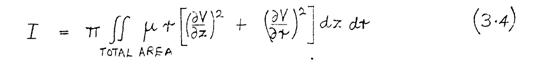
The functional (3.4) is minimised numerically, using the finite element method.

 

B. Vector Potential Program (Dissertation, section 4.1)

 

Calculation of the vector potential allows current-carrying coils to be included in the analysis and the calculation of magnetic flux density. Fig. 4.1 shows a typical magnetic circuit which can be analysed. The data required (Fig. 4.2) comprises three files:

 

COORDS: This specifies the layout of the finite element mesh.

METAL: This specifies the geometry and permeability of the magnetic circuit.

COIL: This specifies the position and excitation of the coil.

The finite element mesh (Fig. 4.4) is generated from the COORDS data, as described in Section 3.1. The peak flux density in the magnetic circuit is calculated; and the axial field distribution is computed from the vector potential values at mesh-points near the axis. The magnetic flux distribution (Fig. 4.5) and the axial field distribution (Fig. 4.6) can be plotted.

The functional for vector potential distributions (Dissertation, section 4.2)

The vector magnetic potential A is defined such that

 

From Maxwell's equations, it follows that A satisfies the differential equation

 

 

where μ is the permeability, and J is the current density, at any point. The solution of (4.2), subject to prescribed boundary conditions, is mathematically equivalent to the minimisation of the functional

 

 

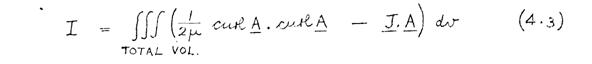
subject to the same boundary conditions. (This is proved in Appendix 2.) The first term in (4.3) can be interpreted physically as the stored magnetic energy.

 

C. Extension of the Finite element Method to deal with Non-linear Media

(Dissertation, Chapter 5)

 

This chapter describes the extension of the finite element method to compute scalar and vector potential distributions in systems with non-linear material properties. This extension enables lenses with saturated pole-pieces and magnetic circuits to be analysed.

The lens geometries chosen as examples in Chapters 3 and 4 will be used again to illustrate the non-linear programs. The only additional data file required is BHVALUES (Fig. 5.1). This specifies the magnetisation curve for the pole-piece material, and the excitations at which the potential distribution is to be computed.

Fig. 5.2 shows a block diagram of the non-linear programs. From the BHVALUES data, the initial permeability μ i (Fig. 5.1) of the pole-piece material is found. Taking μ= μ i for the pole-piece permeability, a linear approximation to the potential distribution is computed, using the scalar or vector potential programs described earlier. A set of non-linear finite element equations is then generated using the BHVALUES data. These non-linear equations are solved by Newton's iteration method (Appendix 8), at each specified excitation. For the first excitation, the linear approximation to the potential distribution provides a starting point for the iteration process. The solution at this excitation then provides a starting point for the iteration process at the next excitation, and so on. At each excitation, convergence to the final solution is usually achieved after two or three iterations.

Equipotential lines, flux distributions, and axial field distributions can be plotted at each. excitation. Figs. 5.3 - 5.6 show typical results- obtained with the non-linear scalar potential program. As the excitation is increased, equipotential lines cut progressively further into the saturated pole-pieces. The half width of the axial field distribution increases, and leakage fields appear in the lens bores. Figs. 5.7 - 5.9 show results obtained with the non-linear vector potential program. As the excitation is increased, flux leaks out of the saturated magnetic material, producing parasitic axial fields in the back bore.

 

The functionals for non-linear scalar and vector potential distributions

(Dissertation, section 5.2)

 

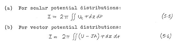
For non-linear scalar potential distributions, the functional to be minimised is

 

 

For non-linear vector potential distributions, the functional to be minimised is

 

 

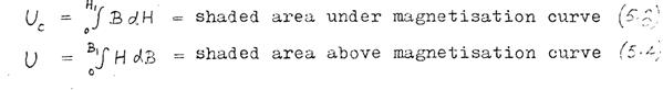
In (5.1), Uc is the complementary magnetic energy per unit volume, and in (5.2), U is the stored magnetic energy per unit volume. These are defined as follows:

Let the magnetic field strength at any point be H l, and let the corresponding flux density be B l.

 

 

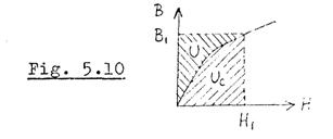
Then

 

Physically, therefore, (5.1) shows that the scalar potential distribution will be such as to minimise the overall complementary magnetic energy, and (5.2) shows that the vector potential distribution will be such as to minimise the overall stored magnetic energy. For the special case of materials with constant permeability, (5.1) and (5.2) reduce to the linear functionals (3.3) and (4.3) respectively.

For a cylindrical polar (z, r, θ) coordinate system with rotational symmetry, the functionals (5.1) and (5.2) become:

 

These functionals are minimised numerically, using the finite element method.

 

 

III. TESTS ON THE ACCURACY OF THE POTENTIAL PROGRAMS

 

This chapter (Chapter 6) describes tests which were used to check the accuracy of the potential programs. These include analytic tests using mathematical models, and comparisons with results of other authors for simple lenses.

A. An analytic test on the scalar potential program:

In this test, the axial potential distribution in the cylindrical electrode system shown in Fig. 6.1 was computed exactly using the following Fourier-Bessel series:

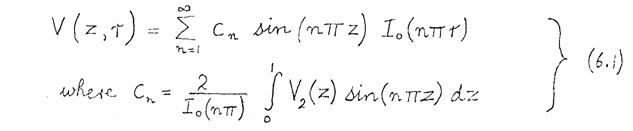
(Io is the modified Bessel function of the first kind of order zero.) The axial potential distribution was then computed using the scalar potential program, and the results were compared with the exact values (Table 6.1). Using a 10 x 10 finite element mesh, the maximum fractional error in the computed axial potential distribution was 0.90%; by using a 20 x 20 mesh, this was reduced to 0.17%. The test was repeated for non-axial mesh points, and a similar accuracy was obtained. The results indicate that the scalar potential program can compute potential distributions to an accuracy of better than 1%. Halving the mesh-length improves the accuracy by a factor of about 5.

 

B. An analytic test on the vector potential program (Dissertation, section 6.2)

In this test, the axial field distribution for the iron-free coil shown in Fig. 6.2 was computed exactly, using the following formula, derived from the Biot-Savart law:

 

 

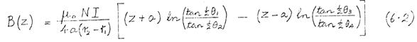
The axial field distribution for the same coil was then computed with the vector potential program, using the two meshes shown in Fig. 6.3. The results are shown in Table 6.2.

The errors which occurred when the mesh boundary was close to the coil (boundary 1) were reduced considerably when the boundary was moved further away (boundary 2). The main source of error was therefore the truncation error due to the proximity of the boundary. When using the vector potential program to analyse iron-free lenses, therefore, the mesh boundary must be a long way from the lens. For iron-shrouded lenses, however, the boundary position is less critical, because there is virtually no field outside the magnetic circuit, and hence the boundary truncation error is negligible. The fractional error in Bz at the centre of the lens was 1.5% using boundary 1; this was reduced to 0.6 by using boundary 2. The vector potential program can therefore compute axial field distributions to an accuracy of better than 1%.

 

C. A test on the non-linear scalar potential program (Dissertation, section 6.4)

Comparison with the results of Bauer (1963)

Bauer estimated the axial field distribution in a magnetic lens under unsaturated and saturated conditions, using a resistance network analogue. Axial field distributions in Bauer's lens (Fig. 3.1) were computed with the non-linear scalar potential program. The computed results (Fig. 6.7) agree well with Bauer's measurements.

 

D. An Experiment to Test the Accuracy of the Non-linear potential programs

(Dissertation, chapter 7)

The potential programs make possible a rapid analysis of the axial field distributions in saturated magnetic lenses. The only published data on such lenses was that of Bauer (1968), who only considered a small degree of saturation. The axial magnetic field in a highly saturated lens was therefore measured experimentally to check the accuracy of the non-linear programs.

 

A modified EM6G (AEI) lens was used for the experiment (Fig. 7.1). To run the lens under highly saturated conditions, the original coil was replaced by a water-cooled coil, capable of running at 20,000 ampturns, with a dissipation of 1.8 kilowatts. The coil was wound in two sections, each consisting of 1000 turns of 19 s.w.g. 'Bicalester' wire, rated for continuous operation at 18000. A thermocouple was embedded at the centre of each section, and the temperature was monitored throughout the experiment. The coil sections were bounded by water-cooled copper end-plates. The windings were insulated from the plates by fibreglass tape.

The axial field was measured using a Hall-effect gaussmeter. (Kindly lent by K.A. Brookes of A.E.I. Scientific Apparatus Division.), with a quoted accuracy of ±2% over its working range of 0 to 3 Wb/m 2. The Hall probe was of 1 mm square cross-section. The probe measured the axial field component, averaged over the area of the Hall element. Since the element width was considerably less than the lens bore diameter, the field value recorded gave a fairly accurate measurement of the axial field distribution. Fig. 7.2 shows the experimental arrangement. Before taking measurements, the Hall probe was centred within the lens bore, by moving the Hall element axially to the position of maximum field strength, at the centre of the pole-piece gap, and then shifting it laterally to minimise the gaussmeter reading. (At the mid-plane of the pole-piece gap in a magnetic lens, Bz is less on the axis than at any other point.)

Experimental plots of the axial field distribution along the entire length of the lens bore at four different excitations were obtained; those for 10,000and 20,000 ampturns are shown in Figs. 7.4 and 7.6. Each plot was obtained directly on the X-Y recorder. The axial scale corresponds one-to-one with the dimensions of the lens. For each excitation, the corresponding field distribution was computed with the non-linear vector potential program. The magnetisation curve assumed is shown in Fig. 7.8. The curve used was that for '0' grade steel, from which the lens was constructed. The computed axial field values are marked by circles in Figs. 7.4 and 7.6. Computer plots of the flux distribution in the magnetic circuit of the lens are also shown. These plots show how the flux lines leak out from the back bore of the lens in a non-linear manner as the excitation is increased.

To obtain a more accurate comparison of the field values in the pole-piece region, the measurements were repeated over an axial range extending from z = -10 mm. to z=+10 mm. The X-Y recorder sweep-rate was increased by a factor of 10 to give an expanded axial scale for these plots. The results are shown in Fig. 7.7. The continuous lines are the Hall probe measurements, and the circles are the computed values. These results indicate close agreement between experimental and computed field values. The parasitic field in the back bore at 20000 ampturns predicted by the computer was within 5% of the measured value. The peak field value, the half-width of the field, and the parasitic field in the back bore at all excitations, were all predicted to within 5%. This indicates that the non-linear programs give sufficiently accurate field values for use in computing the optical properties of saturated lenses.

 

 

IV. COMPUTATION OF THE OPTICAL PROPERTIES OF MAGNETIC LENSES

(Dissertation, Chapter 8)

 

This chapter describes a computer program written to compute the optical properties of any round magnetic lens whose axial field distribution is known.

Description of the program: Paraxial electron trajectories are computed by Runge-Kutta integration of the paraxial ray equation:

in which B(z) is the axial magnetic field distribution, r(z) is the electron trajectory, η is the charge/mass ratio of the electron, and Vr is the relativistically-corrected beam voltage. (The Runge-Kutta formula used to integrate (8.1) is given in Appendix 12. The spherical and chromatic aberration coefficients C_s and C_c, referred to specimen space, are calculated by Simpson's rule integration of the following expressions:

 

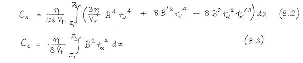
in which z = z 1 is the specimen plane, z = z 2 is the image plane, and r α is the particular solution of (8.1) with initial conditions rα(z 1) = 0 and r'α(z 1) = 1. (Formula (8.1), (8.2), and (8.3) are given in Grivet (1965)). Computational details are given in. Appendix 13.

Two files of data are required to run the program:

AXIALB: This specifies the axial field distribution. This file is usually set up automatically by running one of the potential programs, but any other numerically specified field distribution could be used.

FOCALPTS: This specifies the specimen positions (or ‘working distances') at which the optical properties are required. The output is a table of the following lens properties:

(1) Beam voltage Vr at which the lens has the specified working distance at the given excitation.

(2) Excitation parameter (NI)^2/Vr.

(3) Working distance L.

(4) Objective focal length fo.

(5) Principal plane zp.

(6) Spherical aberration coefficient C_s.

(7) Chromatic aberration coefficient C_c.

(8) Magnetic flux density B_sat the specimen

 

The above quantities are defined in Fig. 8.2. C_s and C_c are normally computed for the condition of infinite conjugates (i.e. with the image plane z = z2 at infinity), since objectives and probe-forming lenses are usually operated in this condition. B_sis an important parameter in the design of probe-forming lenses, where it is usually important to limit the flux density at the specimen to a very low value (see Chapters 9 and 10). However, they can also be computed for finite conjugates if required. The diameters of the aberration discs at the specimen, due to C_s and C_c, are

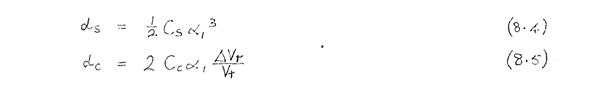
where α 1 is the beam semi-angle at the specimen, and ±ΔVr is the fluctuation in beam voltage.

 

The accuracy of the program has been tested by comparing the computed optical properties of a bell-shaped axial field distribution with exact analytic values calculated from the formulae of Glaser (196). The computed optical properties were all within l% of the exact values. Computed results for simple lenses have also been compared with computed results supplied by a commercial lens manufacturer. Again, agreement between the results was better than 1. These tests are described in Appendix 14.

For an unsaturated lens the optical properties depend on the excitation parameter (NI) 2/Vr. In the case of a saturated lens, however, the properties cannot be expressed in terms of the single variable (NI) 2/Vr; instead, it is necessary to compute the optical properties for a range of absolute values of the excitation NI and the beam voltage Vr. It is then convenient to present each optical property in a separate table, as a function of NI and Vr for each optical property.

Since absolute values of NI and Vr are used in these tables, it is convenient to include a table of the theoretical resolution limit: dmin = 0.43Cs ¼ λ ¾ . The resolution limit, taking chromatic aberration into account, can also be tabulated for any specified beam voltage fluctuation; this enables the resolution of transmission electron microscopes to be estimated, taking into account the electron energy losses which occur in thick specimens.

 

V. THE DESIGN OF A LOW-ABERRATION PROBE-FORMING LENS FOR A SCANNING ELECTRON MICROSCOPE

(Dissertation, Chapter 9)

 

This chapter describes a new design of magnetic probe-forming lens for a scanning electron microscope. In this application, the use of a pinhole lens is essential, to limit the stray magnetic field at the specimen to a small enough value to allow efficient collection of the low-energy secondary electrons. The properties of a wide range of pinhole lenses have been computed with the new programs, and the one which appears to have the smallest aberrations has been built and tested experimentally. The design of the new lens has been. published (Munro 1971). The lens has a spherical aberration coefficient 2.5 times smaller than the widely accepted value quoted by Oatley, Pease and Nixon (1965). This should enable the image recording time in the scanning electron microscope to be approximately halved.

Fig. 9.1 shows the type of pole-piece geometry investigated. Many such pole-pieces were analysed using the scalar potential program described in Chapter 3. This program is particularly well suited to the analysis of pinhole lenses, because the field distribution in the pinhole can be computed accurately by placing a high density of finite elements in the bore region. It is no longer necessary to resort to analytical approximations for the field in the pinhole, as was done by Liebmann (1955b).

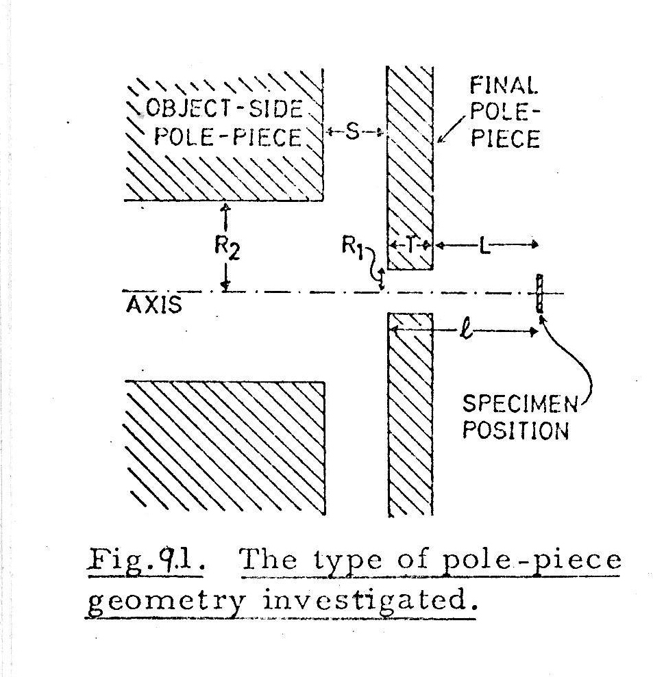
For any given pole-piece geometry, the aberration coefficients C_s and C_c decrease as the working distance l is decreased, so it is desirable to operate the lens at the smallest practicable value of l. Since l = T +L (Fig. 9.l), T and L should both be made as small as possible. If T is made too small, the pole-piece saturates and the stray magnetic field at the specimen becomes too large. If L is made too small, specimen handling becomes difficult. T = 1 mm., L = 2mm., l = 3 mm. are reasonable values, and will be assumed in what follows.

The effect of varying the pinhole bore radius R1 was investigated by computing C_s, C_c and B_s(stray magnetic field at specimen) at l = 3 mm. for three lenses, each with R2=15 mm, and S = 5 mm. The results are shown in Table 9.1. Evidently C_s and C_c are almost independent of R1, whereas B_sdepends critically on R1. It can be shown (Appendix 15) that B_smust be less than about 10 gauss for effective collection of secondary electrons. The pinhole bore radius R1 should therefore be the smallest that can be machined satisfactorily; R1= 0.5 mm. was chosen. Experimental measurements on the prototype lens (Section 9.2) confirm that adequate roundness has been achieved with this bore radius (A method for computing the astigmatism resulting from bore ellipticity is described in Chapter 14.)

Taking l = 3 mm. and R1= 0.5 mm., values of C_s and C_c were computed for many combinations of R2 and S. The results are summarised in Table 9.2. For l = 3 mm., C_c decreases monotonically as R2 is reduced, but C_s has a minimum value when R2 = 15 mm. R2 = 15 mm. was chosen, so as to minimise C_s, since C_s imposes a more fundamental limit on the performance than C_c does. R2 = 15 mm. provides ample space for mounting scanning coils in the large bore. As S is made smaller, C_s and C_c are both reduced. It is convenient however, for mounting an aperture stage and stigmator, to have a fairly large gap, say S = 7.5 mm.; reducing S below this value does not reduce C_s and C_c very significantly. A fairly large gap also limits the flux density in the gap to a small value, thus avoiding saturation in the final pole-piece.

Having deduced suitable dimensions for the pole-pieces, the vector potential program described in Chapter 4 was used to design a magnetic circuit (Fig. 9.2) in which the flux density would be well below saturation level at all points. The final pole-piece has been made conical in shape; this allows the pole-piece to be very thin near the axis, whilst avoiding saturation in the gap region. Fig. 9.3 shows a computer plot of the magnetic flux distribution. Table 9.3 summarises the computed specification of the lens at l = 3 mm. Figs. 9.4 and 9.5 show computed values of C_s and C_c as functions of l.

The lens shown in Fig. 9.2 was built, and C_s and C_c were measured experimentally as functions of l; the results are plotted in Figs. 9.4 and 9.5 for comparison with the computed values. C_s was measured using the grid shadow projection method (Kanaya et al. 1967). C_c was determined experimentally as follows. Defining p = Vr/(NI) 2, measured values of l were plotted as a function of p (Fig. 9.10). Within the limits of error of the experiment, l was a linear function of p. The value of dl/dp was found from the slope of the graph. C_c, as a function of l, is then given by C_c = dl/dp.

The performance of the new lens compared with previous lenses: Oatley, Pease, and Nixon (1965) quoted a value of C_s 20 mm. for a magnetic scanning microscope lens, and this has been widely accepted as a typical value. The new lens has a value of C_s which is 2.5 times smaller than this.

 

VI. MAGNETIC PROBE-FORMING LENSES FOR OTHER APPLICATIONS

 

This chapter describes the application of the new programs to the design of X-ray microanalyser lenses, iron-free mini-lenses, and a long-working-distance lens.

 

A. X-ray nicroanalyser lenses:

The design requirements for X-ray microanalyser lenses, which have been discussed by Mulvey (1959) and Duncumb (1969), are:

(1) C_s should be as small as possible, since the current obtainable in a probe of given diameter is proportional to l/Cs (2/3). If C_s can be halved, the probe current can be increased by a factor of 1.6, giving a corresponding increase in X-ray emission.

(2) For the analysis of ferromagnetic specimens, the stray magnetic field at the specimen must be small enough not to defocus the probe.

(3) X-rays must be collected over a wide range of emission angles. To achieve this, the final pole-piece may be tapered to allow X-rays to travel at large angles outside the lens, or the inner bore may be tapered so that X-rays can be collected through the bore.

(4)The magnetic circuit should be designed leaving as much space as possible for mounting the X-ray collection system.

These requirements impose considerable restrictions on the lens geometry, so it is necessary to use complicated pole-piece profiles. The ease with which the new programs handle complicated pole-piece shapes will be apparent from the two examples given here.

The first design (Fig. 10.1) incorporates the following features:

(1) The X-rays are collected outside the lens. The final pole-piece is tapered, to allow X-ray take-off angles of up to 20°.

(2) At a radius of 4 cm., the final pole-piece is cut right back, to provide space for the X-ray collection system.

(3)The lens bore has an inner diameter of 4 cm. This provides adequate space for scanning coils and a stigmator.

(4) The magnetic circuit has been designed to avoid saturation in the back bore. At NI = 1078 ampturns, the peak flux density in the back bore is 1.56 Wb/m2, which is low enough to prevent flux leakage. If the lens were to be operated at higher excitations, flux leakage could be avoided by thickening the back bore.

The optical properties have been calculated for a range of excitations. With the specimen at the optimum position of L = 0 mm. (i.e. just outside the final pole-piece), C_s = 20.7 mm. and C_c = 15.3 mm., with a stray magnetic field at the specimen of B_s= 13 gauss. This compares favourably with the design of Mulvey (1959) for which C_s=30mm.

The second design, shown in Fig. 10.2, has the following features:

(1) The lens is designed to allow collection of the X-rays through the lens bore. The range of angles which can be collected is 64° to 90°, with the specimen situated at a maximum distance of 10 mm. outside the final polo-piece.

(2) The peak flux density in the magnetic circuit is very low. (Bm = 0.52 Wb/m2 at NI = 1140 ampturns.) The excitation could be increased to 2500 ampturns before the onset of saturation, and the lens could therefore be used with high beam voltages, up to about 150 kV. This could be very useful, since a high beam voltage produces a wide spectrum of X-rays.

The optical properties have been calculated for a range of excitations. The magnetic field at the specimen is much higher than in the previous design. For ferromagnetic specimens, therefore, it would be necessary to place the specimen at the maximum working distance of L = 10 mm. For non-magnetic specimens, however, the specimen could be immersed in the magnetic field, at L = 0 mm. At this working distance, the aberrations are very low: C_s 3.5 mm., and C_c = 4.5 mm. This lens is thus a good design for the analysis of non-magnetic specimens.

 

B. The design of iron-free mini-lenses

An iron-free mini-lens (Le Poole 1964) consists simply of a coil of wire a few millimetres in diameter, wound on a conical former (Fig. 10.3). The coil is generally surrounded by a water-cooled copper jacket. Such lenses are particularly useful for X-ray microanalysers, because they permit a larger range of take-off angles than iron-shrouded lenses. Their main disadvantage is that they are prone to astigmatism, but this can usually be corrected with a stigmator.

The properties of such lenses can be computed with the vector potential program. A typical example is shown in Fig. 10.4. The optical properties of this lens (Table 10.3) compare favourably with those of iron-shrouded lenses. For example, at a working distance of L = 4 mm., C_s = 23.7 mm., C_c = 15.8 mm., and B_s= 24 gauss.

 

C. A new design of probe-forming lens with low

aberrations at long working distances

To obtain the highest resolution in. the canning electron microscope, a very small working distance (about 3mm.) is required. (see Chapter 9). However, it is sometimes essential to use a very long working distance, say 20-30 mm. The scalar potential program has been used to design a lens (Fig. 10.5a) which is well suited to this application. Fig. 10.5c shows C_s as a function of L for this lens. The corresponding curve for the lens of Chapter 9 is plotted for comparison. Whilst the lens of Chapter 9 has a smaller C_s at small values of L, the long-working-distance lens has a much smaller C_s at large values of L. This reduction in C_s was achieved by tapering the pole-pieces (Fig. 10.5a) to produce an axial field distribution with a very long tail (Fig. 10.5b) The optical properties of the long-working-distance lens at L = 30 mm. are:

Excitation parameter (NI) 2/Vr = 36.8 amp2/volt.

Spherical aberration C_s = 159 mm.

Chromatic aberration C_c = 49 mm.

Focal length fo = 57 mm.

 

 

VII. THE DESIGN OF ELECTROSTATIC LENSES FOR USE WITH

FIELD-EMISSION CATHODES

(Dissertation, Chapter 11)

 

Crewe (1968) has designed a field--emission gun which provides a high-brightness electron probe of very small diameter, suitable for use in a scanning transmission electron microscope. Crewe's gun consists of a field--emission cathode followed by a two-electrode electrostatic lens. In an attempt to minimise the lens aberrations, Crewe has used very complicated electrode shapes, which have to be made on a numerically-controlled lathe. In this chapter, it is shown that it is possible to design. A lens with a performance significantly better than Crewe's lens, using much simpler electrodes.

Fig. 11.1 shows the type of lens investigated. It consists of two electrodes, at potentials of V1 and V0 volts measured relative to the cathode. The distance between the outside of the electrodes is L, the distance of the cathode from the first electrode is S1, and the distance from the second electrode to the focussed spot is S0. The optical properties of the lens depend on the ratio V0/V1, and on the geometry of the electrodes.

 

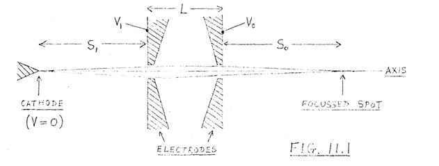
The lenses which have been analysed are shown in Fig. 11.2. The 'ideal Crewe lens' is Crewe's design; the other five lenses are the author' s own designs. In order to obtain a comparable set of results, all the lenses have the same overall length L = 20 mm. (This value is the same as in Crewe's design; this enabled a direct comparison to be made with his published results.)

Crewe maintained that the aberration in an electrostatic lens generally occurs near the electrode apertures, where the field usually changes rapidly. He therefore designed his lens so that the field would be zero near both apertures. His lens has the following axial potential distribution:

which has the desired property that

The potential distribution (11.1) is realised by making the

electrodes follow the analytic curve:

This complicated electrode structure (Fig. 11.2a) is made on a numerically-controlled lathe.

The 'approximate Crewe lens' (Fig. 11.2b) is similar to Crewe's design, but the analytic. curve (11.3) has been approximated by a few straight-line segments. This lens could be made easily on an ordinary lathe. The 'simplified Crewe lens' (Fig. 11.2c) represents a further simplification, in which each electrode has only one tapered portion. In the other three designs (Figs. 11.2d, e, f), one or both of the electrodes is replaced by a flat plate with a hole in it.

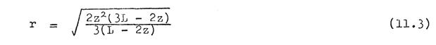
Computation of the lens properties: For the ideal Crewe lens, the axial potential distribution V(z) was obtained from (11.1). The axial potential distributions in the other five lenses were computed using the scalar potential program. Paraxial trajectories were computed by Runge-Kutta integration of the paraxial ray equation:

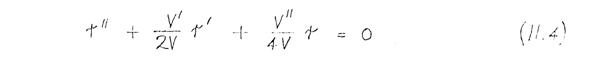
and the spherical and chromatic aberration coefficients, referred to object space, were computed by Simpson's rule integration of the following expressions:

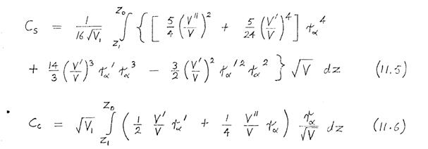
wherein r α(z) is the solution of (11.1) with initial conditions r α(z 1) = 0 and r' α(z 1) = 1. Formulae (11.4), (11.5), (11.6) are given in Grivet (1965). The magnification of the lens was calculated from the formula:

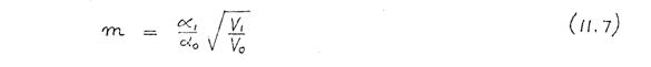
where α 1 and α 0 are the off-axis angles in object and image space.

The probe diameter depends on four factors:

(1) Spherical aberration

(2) Chromatic aberration

(3) Effective source diameter at cathode

(4) Diffraction

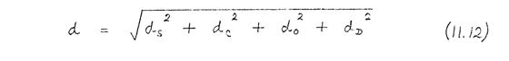
The image diameters, due to each of these factors, are:

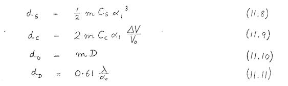
where ±ΔV is the variation in cathode emission potential, D is the effective source diameter, and λ is the wavelength of the electrons at a potential V 0. The overall probe diameter can then be estimated from the following formula:

The corresponding probe current is given by

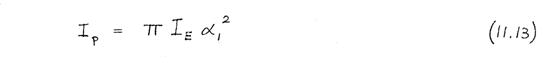
where I E is the emission current per steradian.

The optical properties of each lens were computed at a constant image distance of S 0 = 10 mm., and a constant first anode potential of V 1 = 1 kV. Values of S 1, C_s, C_c, and m were computed for various values of V 0/V 1. Curves for C_s and C_c are shown in Figs. 11.6 and 11.7. In each graph, the dotted curve represents the results both for the ideal Crewe lens and for the approximate Crewe lens, which were indistinguishable. The computed results agreed perfectly with Crewe's published values. The best lens will be the one with the smallest values of C_s and C_c for any given value of m, because this lens will produce the smallest aberration discs for any given Gaussian probe diameter.

The minimum probe diameter for each lens has been calculated from (11.12), assuming an effective source diameter of D = 100 angstroms and a fluctuation in cathode emission potential of ΔV = ±0.1 volts. (These are widely accepted as typical values.) The minimum probe diameter for each lens under these conditions is plotted in Fig. 11.8.

Discussion of the results: The ideal Crewe lens, the approximate Crewe lens, and the simplified Crewe lens have almost identical axial potential distributions, and therefore their optical properties are all very similar. The computed performance of 'the flat-plate lens was inferior to that of the Crewe lenses; this was an expected result, because the field changes rapidly near both apertures. Fig. 11.8 shows that a reduction of about 16% in the minimum probe diameter can be expected by using hybrid lens 1 in preference to the Crewe lens. In addition to having simpler electrodes than the Crewe lens, hybrid lens 1 has the practical advantage of a wider gap between the electrodes, and therefore the lens can be operated at higher voltages without breakdown.

 

 

VIII. THE DESIGN OF SATURATED OBJECTIVE LENSES FOR TRANSMISSION ELECTRON MICROSCOPES

(Dissertation, Chapter 12)

 

This chapter presents computed optical properties for three objective lenses for transmission electron microscopes. All three lenses have been analysed under saturated conditions. The first is the Riecke-Ruska lens, which is widely accepted as one of the best published designs of objective lenses. The other two lenses are new designs, with optical properties as good as those of the Riecke-Ruska lens, However, the new lenses offer the practical advantages of lower heat dissipation and much simpler specimen manipulation. Both lenses can be used with beam voltages of up to 1000 kV. At 1000 kV, they have resolution limits of 0.97 A and 1.20 A respectively.

 

A. The Riecke-Ruska Lens

The Riecke-Ruska lens was designed by Riecke (1962) and Ruska (1962). The magnetic circuit was designed to avoid stray fields in the lens bores at very high excitations. The dimensions of the pole-pieces are S = 2.5 mm., D1 = D2 = 2 mm. The flux distributions in this lens, and the corresponding axial fields, were computed at excitations of NI = 5000, 10000, 15000, and 20000 ampturns. That for NI = 20000 ampturns is shown in Fig. 12.4. (The magnetisation curve used for the pole-piece material is shown in Fig. 7.8.) In computing these distributions, use was made of the symmetry plane of the lens, to halve the number of mesh-points required. The peak flux density in the magnetic circuit is indicated on the computer plot. The axial field plots confirm that there is negligible stray field in the lens bores, even at 20000 ampturns. It is important to avoid such stray fields, for two reasons:

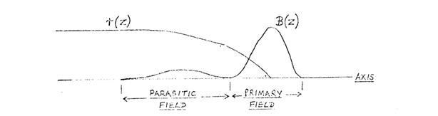
(a) Stray fields have an adverse effect on the aberration coefficients. The formula for C_s contains a B 4r 4 term, and r is relatively large in the back-bore (as shown in the diagram below), so that even a small value of B has a serious effect.

 

(b) The stray fields in the bores are unlikely to be rotationally-symmetric, due to local variations in magnetic properties, and this may produce astigmatism.

The properties of the Riecke-Ruska lens at 50 kV, 200 kV, and 1000 kV are summarised in Table 12.7. The excitations shown in Table 12.7 are those which provide the best resolution at each of the specified beam voltages. 'dmin' is the theoretical resolution limit, and 'dmin*' is the resolution limit obtainable for a beam voltage fluctuation of ΔVr/Vr = 10 -5 The computed results confirm that the Riecke-Ruska lens has excellent optical properties. At 1000 kV, the resolution limit is less than 1 angstrom.

Table 12.7 Summary of properties of Riecke-Ruska lens

Vr = 50 kV. V r = 200 kV. Vr = 1000 kV.

NI = 10000 NI = 10000 NI = 20000

zf = -1.11 mm. zf = 0.15 mm. zf = 1.32 mm.

fo = 1.55 mm. fo = 1.57 mm. fo = 3.16 mm.

C_s = 0.48 mm. C_s = 0.65 mm C_s = 1.29 mm.

C_c = 0.95 mm. C_c = 1.03 mm. C_c = 1.95 mm.

dmin = 2.27 A. dmin = 1.46 A . dmin = 0.95 A.

dmin* = 2.66A. dmin* = 1.87 A . dmin* = 1.80 A

 

 

B. A new design of objective lens with the pole-pieces

at the centre of the magnetic circuit

 

Figs. 12.7 and 12.8 (LENS 1) show the design of the lens. The pole-piece dimensions are S = 2 mm., D1 = 6 mm., and D2 = 2 mm. Flux distributions have been calculated for NI = 5000, 10000, 15000, and 20000 ampturns. Stray fields in the lens bores are avoided at all excitations up to 20000 ampturns. This has been achieved by tapering the back bores at 45°, so that the bore radii away from the pole-piece region are large enough to prevent saturation. Saturation effects are then confined to the vicinity of the pole-pieces. The design of the lens requires the coil to be wound on a V-shaped former; this does not involve any practical difficulty.

The large diameter of the left-hand bore (Dl = 6 mm.) permits a versatile specimen stage to be fitted. The small diameter of the right-hand bore (D2 = 2 mm.) enables a high value of peak axial flux density Bo to be achieved, in relation to the flux density Bp in the gap.. (It was shown by Liebmann (1955a) that Bo/Bp increases as D2/Dl is reduced.) The higher the value of Bo/Bp, the greater is the focussing power for any given excitation.

The detailed optical properties are summarised in Table 12.14. The excitations shown in Table 12.14 are the optimum values for the specified beam voltages. The resolution limit of the new lens at 1000 kV is less than 1 angstrom. Comparison of Tables 12.7 and 12.14 shows that the optical properties of the Riecke-Ruska lens and those of the new lens are almost identical; however, the new lens has the practical advantage that specimen handling is much simpler. Also, the excitation required at high voltages is lower, because of the asymmetry of the lens bores. The heat dissipation is therefore reduced.

Table 12.14 Summary of properties of Objective Lens 1

Vr = 50 kV. Vr = 200 kV. Vr = 1000 kV

NI = 5000 NI = 10000 I = 15000

zf = -0.92 mm. zf = -1.17 mm. zf = 0.56 mm.

fo = 1.42 mm. fo = 2.26 min. fo = 3.31 mm.

C_s = 0.55 mm. C_s = 0.94 mm. C_s = 1.42 mm.

C_c = 0.95 mm. C_c = 1.48 mm. C_c = 2.24 mm.

dmin = 2.35 A. dmin = 1.60 A. dmin = 0.97 A.

dmin* = 2.70 A dmin* = 2.21 A. dmin* = 1.97 A.

 

 

C. A new design of objective lens with the pole-pieces at one end of the magnetic circuit

For many applications, it is convenient to use an objective lens with pole-pieces at one end of the magnetic circuit, since this makes specimen handling simpler than if the pole-pieces are located centrally. It was seen in Chapter 7 that the EM6G lens was unsuitable for operation at very high excitations, because there was excessive flux leakage from the back bore. The new lens (Figs. 12.11 and 12.12, LENS 2) has been designed to overcome this difficulty. The flux plots show that the problem of saturation has been solved by increasing the thickness of the back bore; there is negligible flux leakage at excitations up to 20000 ampturns. Table 12.21 summarises the performance. The optical properties are similar to those of the previous lens.

Table 12.21 Summary of properties of Objective Lens 2

Vr = 50 kV. Vr = 200 kV. Vr = 1000V.

NI = 20000 NI = 20000 NI = 20000

zf = -1.43 mm. zf = -0.03 mm. zf = 2.84 mm.

fo = 1.82 mm. fo = 1.90 mm. fo = 3.47 mm.

C_s = 0.47 mm. C_s = 0.94 mm. C_s = 3.36 mm.

C_c = 0.88 mm. C_c = 1.23 mm. C_c = 2.65 mm.

dmin = 2.26 A. dmin = 1.60 A. dmin = 1.20 A.

dmin* = 2.60 A. dmin* = 2.05 A. dmin* = 2.03 A.

 

IX. THE DESIGN OF FOCUSSING SYSTEMS FOR SPECIAL APPLICATIONS

(Dissertation, Chapter 13)

 

This chapter describes the application of the new computer programs to the design of three special types of focussing systems, namely superconducting lenses, devices for focusing hollow electron beams, and electron energy filters.

A. Design of superconducting lenses

 

Superconducting lenses can be used as objective lenses in transmission electron microscopes. In this application, they offer the following advantages over conventional types:

(1) The lens current is very stable (about 1 part in 10 7) ; which means that chromatic aberration due to lens current fluctuation is negligible.

(2) Very high axial flux densities can be achieved (about 10 Wb/m 2). This enables electron beams of several million volts to be focused easily-.

(3) The axial magnetic field can be confined to a short axial length by superconducting shielding cylinders. This makes the aberrations very small.

(4) The current density in the windings can be extremely high, and so a superconducting lens is much smaller than a conventional lens of the same strength.

For these reasons, superconducting lenses will be a topic of increasing importance during the next few years. Many designs for superconducting lenses have already been published, e.g. Fernandez-Moran (1966), Ozasa et al. (1966), Genotel et al. (1968), Bonjour and Septier (1968), Dietrich et al. (1969), and Trinquier and Balladore (1970). All these lenses were designed by trial-and-error methods, because no methods were available for computing their properties before they were built. The new programs, however, can compute the properties of any superconducting lens, for the following reasons:

(1) In superconducting lenses, the excitation is so high that the position of the coil has considerable influence on the lens properties. The direct effects of the coil, which could not be dealt with previously, can now be calculated using the vector potential program.

(2) The magnetic materials in a superconducting lens are usually highly saturated. The saturation effects can be computed with the non-linear programs.

(3) The effect of superconducting shielding cylinders can now be computed for the first time.

 

A couple of examples will be given to illustrate these points.

Fig. 13.1 shows a lens of the type designed by Fernandez-Moran (1966). It consists of a coil of superconducting wire, surrounded by an iron yoke. The flux distribution in this lens at 50,000 ampturns has been computed with the non-linear vector potential program. The iron yoke is highly saturated, so the position of the coil has a considerable influence on the axial field distribution. The effects of altering the position of the coil or modifying the shape of the magnetic circuit could be investigated very easily.

Fig. 13.2 shows a lens of the type designed Dietrich et al. (1969). It consists of a coil of superconducting wire A, an iron yoke B, and two superconducting cylinders C. The superconducting cylinders completely exclude magnetic flux by the Meissner effect (Fig. 13.2a), (see, for example, Bleaney and Bleaney (1965)) so that the axial magnetic field is confined to a short axial length (Fig. 13.2b). The Meissner effect is simulated by setting the permeability of the superconducting cylinders equal to zero. Above a critical surface field strength Hc, the Meissner effect begins to break down, and the flux density B penetrates into the superconducting material. If the relationship between H and B for the material is known, the onset of breakdown of the Meissner effect can be treated as a saturation phenomenon, and investigated with the non-linear programs.

 

B. Design of a focusing device for imparting a spin to a hollow beam of electrons

The scalar potential program has been used to design a magnetic focussing device for imparting a spin to a hollow beam of electrons. The device has been used by Mills (1971) in an apparatus for generating millimetre electromagnetic waves

Fig. 13.3a shows the focussing device originally developed by Mills. It consists of an iron plate A with a central hole, within which a small iron disc B is supported coaxially by four wires (Fig. 13.3b). An axial magnetic field is produced on each side of the plate A by means of the pole-pieces C, energised by the coils D. The coils are energised in opposite directions, so that all the axial flux converges onto the central disc B. In this way, a radial magnetic field is set up in the annular gap between the disc B and the plate A.

A hollow beam of electrons travels axially through the device. Initially the beam has no spin, and is therefore unaffected by the axial magnetic field. As the beam passes through the gap, however, the radial field in the gap imparts a spin to the electrons. The beam then continues to spin, the required inward acceleration being provided by the axial field.

Magnetic field distributions in the gap region were computed for various gap geometries, using the scalar potential program. A typical example is shown in Fig. 13.4. Electron trajectories were then computed (Mills 1971), and the design of Fig. 13.4 was found to perform satisfactorily. The effect of removing the

central disc was then investigated (Fig. 13.5). Figs 13.4 and 13.5 show that the magnetic field at the beam radius r = r b remains virtually unchanged when the central disc is removed. This indicates that the device will work equally well without the central disc. Mills built the design shown in Fig. 13.5, and found that it performed as predicted. The omission of the central disc simplified the construction and alignment.

 

C. Design of electron energy filters and energy analysers

 

Bunting (1971) has used the scalar potential program, and a trajectory program written by the author, to compute the properties of a wide range of electrostatic energy filters. The filter was required for use in a scanning electron diffraction apparatus, to remove electrons which had lost energy in passing through the specimen. Many complicated designs for such filters had been published previously. The use of the scalar potential program led to the design of a simpler and more effective filter.

Fig. 13.6 shows the type of filter investigated. It consists of two outer electrodes at anode potential, and a central electrode which can be biassed a few volts positive or negative relative to cathode potential. Electrons enter through an aperture, and are retarded as they approach the central electrode. Electrons which have lost energy in passing through the specimen are unable to cross the saddle potential at the central electrode. Electrons which have not lost energy do get through, and are accelerated towards the exit aperture.

Axial potential distributions and electron trajectories were computed for many such filters. The computed results showed that the shape of the outer electrodes is unimportant, but that the trajectories depend critically on the shape of the central electrode. This is because the electrons are moving slowly near the central electrode, and hence the radial fields at the edge of the central hole have a considerable focussing effect. Trajectory plots for two central electrode shapes are shown in Fig. 13.7 (Reproduced from Bunting (1971) with permission).

The electron energies, relative to the saddle potential, are marked on the plots. The inter-electrode potential was 100 kV. The trajectories in Fig. 13.7a are for a central electrode consisting of a flat plate with a hole in it. The trajectories in Fig. 13.7b relate to the modified central electrode shown in Fig. 13.6, in which each end of the central hole has a conical taper. This taper reduces the radial field near the hole, and hence reduces the radial dispersion of the trajectories (Fig. 13.7b). The trajectories of Fig. 13.7b are superior to those of Fig. 13.7a, because a larger entrance aperture can be used without fear of losing any of the transmitted electrons. The design of Fig. 13.6 was built, and its. performance confirmed the computer predictions.

The filter could be used as an electron energy analyser, by varying the bias on the central electrode to select the cut-off potential. The energy resolution obtainable is approximately 1 part in 10 5 of the potential difference between the electrodes.

 

 

 

X. COMPUTATION OF THE ABERRATIONS RESULTING FROM ELLIPTICAL DEFECTS IN ELECTRON LENSES

(Dissertation, Chapter 14)

 

This chapter describes the extension of the finite element method to compute the astigmatism resulting from bore ellipticities in electron lenses. Previous calculations on ellipticities, by Bertein (1947 and 1948), Sturrock (1951) and Archard (1953), were confined to lenses with very simple pole-piece shapes. The method described in this chapter, on the other hand, can deal with lenses of any shape.

A program based on the new method has been used to compute the effects of bore ellipticity for the pinhole lens of Chapter 9. The computed results show that the machining tolerance for the roundness of the large bore is far more stringent than that for the pinhole bore.

 

A. The perturbation potential resulting from an arbitrary

perturbation of pole-piece geometry

 

Let S 0 be a point on the surface of the unperturbed pole-pieces, and let S 1 be the corresponding point on the perturbed pole-piece surface (Fig.14.1). Let the displacement vector from S 0 to S 1, be δn(S 0). Let P be a general point. Let V 0(P) be the potential distribution in the unperturbed lens, and let δV(P) be the perturbation potential resulting from the pole-piece displacement δn(S 0). ( This section is a simplified form of the theory of Sturrock (1951).) Then the potential distribution in the perturbed lens is

 

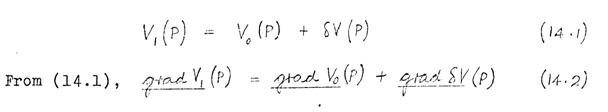
Using Taylor's theorem, and neglecting terms in ∇ n² and above

Inserting (14.1) and (14.2) into (14.3), and neglecting second-order terms, gives:

Now V 1(S 1) = V 0(S 0), since the potential on the pole-piece surface is the same in the perturbed lens as in the unperturbed lens. Hence (14.4) becomes:

In (14.5), grad V 0 ( S 0 ) is the potential gradient at the surface of the unperturbed pole-pieces, and δn( S 0 ) is the displacement vector. Hence the perturbation potential δV(S 0) at the pole-piece surface can be calculated from (14.5).

 

At all points P between the pole-pieces, V 0(P) and V 1(P) satisfy Laplace's equation. It follows from (14.1) that δV(P) also satisfies Laplace's equation, i.e.

The solution of (14.6), subject to the boundary conditions (14.5), therefore yields the perturbation potential δV(P).

 

B. The perturbation potential resulting from a lens-bore ellipticity

 

Suppose that one of the lens bores has an elliptical defect (Fig. 14.2), such that its radius is

where ε is the magnitude of the ellipticity. Then the displacement vector (defined in Section 14.1) is

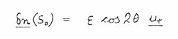
(14.7)

 

 

and the potential gradient at the pole-piece surface is

 

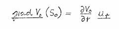
(14.8)

 

where u r is a unit vector in the r-direction. Inserting (14.7) and (14.8) into (14.5) gives the perturbation potential at the pole-piece surface:

Fig. 14.3 shows a lens in which one bore has an elliptical defect; the other bore is round. The perturbation potential at the pole-piece surface, which is given by (14.9), is indicated in Fig. 14.3. From (14.6) the potential perturbation between the pole-pieces satisfies Laplace's equation, i.e.

 

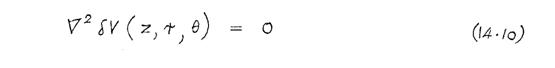
C. The functional for the perturbation potential due to a lens-bore ellipticity

 

The solution of (14.10), subject to the boundary conditions (14.9), is mathematically equivalent to the minimisation of the functional

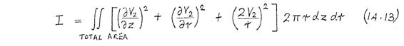
subject to the same boundary conditions. (This is a special case of the functional derived in Appendix 1.) Since the boundary conditions (14.9) have an angular variation proportional to cos 2θ, the solution has the same angular dependence, i.e.

where V 2 is a function of z and r only. Substituting (14.12) into (14.11) gives

Since δV(z,r,θ) satisfies the boundary conditions (14.9), it follows from (14.12) that V 2(z,r) satisfies the following boundary conditions:

 

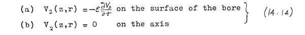
These boundary conditions are illustrated in Fig. 14.4.

 

The minimisation of the functional (14.13), subject to the boundary conditions (14.14), yields the perturbation potential distribution V 2(z,r). The functional is minimized numerically, using the finite element method.

 

D. Outline of the program for computing the astigmatism

resulting from bore ellipticities

 

A block diagram of the program is shown in Fig. 14.6, which is self-explanatory.

Since the astigmatism coefficient is proportional to the absolute machining error ε (defined in equation (14.6a)), it is convenient to compute the normalised astigmatism coefficient, i.e. the astigmatism coefficient per unit machining error. Two normalised astigmatism coefficients are computed:

C_eA, for a machining error in the object-side bore.

C_eB, for a machining error in the image-side bore.

C_eA and C_eB can be computed for any specified range of working distances.

 

E. Computed astigmatism coefficients for a range of pinhole lenses

 

The program has been used to compute the effects of lens-bore ellipticity in the new design of magnetic pinhole lens described in Chapter 9. The dependence of the astigmatism coefficients on the pinhole-bore radius has been investigated by analysing three lenses, each with a large-bore radius R 2 = 15 mm. and a gap S = 7.5 mm., for three different values of the pinhole-bore radius R 1. The normalised astigmatism coefficients C_eA andC_eB for each lens are plotted in Fig. 14.7.C_eA is the astigmatism coefficient for ellipticity of the large bore, and C_eB is the corresponding coefficient for the pinhole bore.

The computed results show that the machining tolerance is far more stringent for the large bore than for the pinhole bore. As an example, for the lens with R 1 = 0.5 mm. at l = 3 mm., an ellipticity of ±1 micron in the large-bore radius produces an astigmatism coefficient of C_e= 57 microns; an ellipticity of 1 micron in the pinhole-bore radius, however, results in C_e= 0.02 microns. This is a useful practical result, because the pinhole bore is much more difficult to machine accurately than the large bore. Physically, the astigmatism resulting from ellipticity of the pinhole bore is so small because very little focussing action occurs in the pinhole.

In practice, the astigmatism can be partially or wholly compensated with a stigmator. If the maximum value of astigmatism which the stigmator can correct is known, then absolute machining tolerances for the bore roundness of any lens can be computed with the new program

 

Editor’s Note on Chapters 15, 16 and 17 of Munro’s Dissertation

 

Chapters 15 and 16 describe work relating to the properties of secondary electron detectors for the scanning electron microscope. The finite element method is not used for this work and is, therefore, omitted from this presentation. Chapter 17, also omitted, contains proposals for future work (see Introduction).

 

REFERENCES

 

ARCHARD, G.D. (1953) J. Sci. Inst ., 30, 352.

ARLETT, P.L., BAHRANI, A.K. and ZIENKIEWICZ, O.C. (1968) Proc. I.E.E., 115, 1762.

BALLANTYNE, J.P., YAKOWITZ, H., MUNRO, E. and NIXON, W.C. (1971) Proc. 25th Anniversary Meeting of the Electron Microscopy and Analysis Group, Institute of Physics, London, 194.

BANBURY, J.R. and NIXON, W.C. (1969) J. Sci. Inst., Series 2, 2, 1055.

BANBURY, J.R. (1970) Ph.D. Thesis, Cambridge.

BAUER, M. (1968) Sci. Inst., Series 2, 1, 1081.

BERTEIN, F. (1947) Ann. de Radioel., 2, 10.

BERTEIN, F. (1948) Ann. de Radioel., 3, 11.

BLEANEY, B.I. and BLEANEY, B. (1965) 'Electricity and Magnetism', 2nd Edition, Clarendon Press, Oxford.

BONJOUR, P. and SEPTIER, A. (1968) Proc. Fourth Eur. Conf. for Electron Microscopy, Rome, 1, 189.

BROERS, A.N. (1969) J. Sci. Inst., Series 2, 2, 273.

BUNTING, C.D. (1971) Proc. 25 th Anniversary Meeting of the Electron Microcopy and Analysis Group, Institute of Physics, London, 90.

CREWE, A.V. et al. (1968) Rev. Sci. Inst., 39, 576.

DIETRICH, I., PFISTERER, H. and WEYL, R. (1969) Z. angew. Phys. 28, 35.

DORSEY, J.R. (1969) Adv. in Electronics and Electron Physics, Suppl. 6, 291.

DUGAS, J., DURANDEAU, P. and FERT, C. (1961) Revue d'Optique, 40, 277.

DUNCUMB, P. (1969) J. Sci. Inst., Series 2, 2, 553.

DURANDEAU, P. and FERT, C. (1957) Revue d'Optique, 36, 205.

EL-KAREH, A.B. (1969) Proc. Tenth Int. Symposium on Electron, Ion and Laser Beam Technology, Gaithersburg, Maryland, 393.

FERNANDEZ-MORAN, H. (1966) Proc. Sixth Int. Congress for Electron Microscopy, Kyoto, 1, 147.

GÉNOTEL, D. et al. (1968) Proc. Fourth Eur. Conf. for Electron Microscopy, Rome, 1, 187.

GLASER, W. (1956) Handbuch der Physik, 33, 123.

GRIVET, P. (1965) 'Electron Optics', Pergamon Press, Oxford.

HEATH, A.C. (1966) Private Communication.

HEDDLE, D.W.O. (1969) J. Sci. Inst., Series 2, 2, 1046.

HEDDLE, D.W.O. (1970) J. Sci. Inst., Series 2, 3, 552.

JONKER, J.L.H. (1951) Philips Research Reports, 6, 372.

KAMMINGA, W., VERSTER, J.L. and FRANCKEN, J.C. (1968) Optik, 28, 442.

KANAYA, K. et al. (1967) Bull. Electrotech. Lab., 31, 17.

KIRSTEIN, P.T. and HORNSBY, J.S. (1964) I.E.E.E. Trans. on Electron Devices, 11, 196.

LENZ, F. (1950) Z. angew. Phys., 2, 448.

LE POOLE, J.B. (1964) Proc. Third Eur. Conf. for Electron Microscopy, Prague. Supplementary Pages.

LIEBMANN, G. and GRAD, E.M. (1951) Proc. Phys. Soc., 64B, 956. LIEBMANN, G. (1953) Proc. Phys. Soc., 66B, 448.

LIEBMANN, G. (1955a) Proc. Phys. Soc., 68B, 679.

LIEBMANN, G. (1955b) Proc. Phys. Soc., 68B, 682.

MILLS, W.P.C. (1971) Ph.D. Thesis, Cambridge.

MULVEY, T. (1959) J. Sci. Inst., 36, 350.

MULVEY, T. (1967) 'Focusing of Charged Particles', Academic Press, 1, 469.

MUNRO, E. (1970) Proc. Seventh Int. Congress for Electron Microscopy, Grenoble, 2, 55.

MUNRO, E. (1971) Proc. 25th Anniversary Meeting of the Electron Microscopy and Analysis Group, Institute of Physics, London, 84.

OATLEY, C.W., PEASE, R.F.W. and NIXON, W.C. (1965) Adv. in Electronics and Electron Physics, 21, 181.

OZASA, H. et al. (1966) Proc. Sixth Int. Congress for Electron Microscopy, Kyoto, 1, 149.

READ, F.H. (1969a) J. Sci. Inst., Series 2, 2, 165.

READ, F.H. (1969b) J. Sci. Inst., Series 2, 2, 679.

RIECKE, W.D. (1962) Proc. Fifth Int. Congress for Electron Microscopy, Philadelphia, 1, KK-5.

ROSE, A. (1948) Advances in Electronics, 1, 131.

RUSKA, E. (1962) Proc. Fifth Int. Congress for Electron Microscopy, Philadelphia, 1, A-1.

STURROCK, P.A. (1951) Phil. Trans. Roy. Soc., 243A, 387.

TRINQUIER, J. and BALLADORE, J.L. (1970) Proc. Seventh Int. Congress for Electron Microscopy, Grenoble, 2, 97.

ZIENKIEWICZ, O.C. and CHEUNG, Y.K. (1965) The Engineer, 220, 507.

ZIEIKIEWICZ, O.C. (1967) 'The finite element method in structural and continuum mechanics', McGraw-Hill, London.