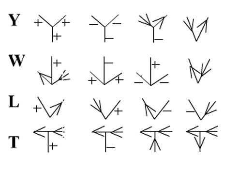
If we make these restrictions (Note they can be lifted), it turns out hat there are only four types of juncttion to be considered. These are L-junctions, Y- or fork-junctions, W- or arrow-junctions and T-junctions.
Constraint Propagation in line labelling
One of the most elegant AI applications of constraint satisfaction is junction and line labelling in computer vision, an example of symbolic, rather than numeric, constraint propagation.
Human beings have been shown to have an in-built ability to make sense of the 3D shape implications of 2D line drawings, especially polyhedra. This ability comes about because there are provably very few ways of interpretating line drawings. This ability has been captured in machine vision programs, the simplest of which we outline now.
Consider objects which:
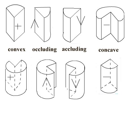
Let us now look at edges on a polyhedral object. These can be convex, concave or occluding (two sorts), so there are four ways of labelling a line. We label these with a plus, a minus, or left or right arrows (by convention the solid face is to right of edge when traversed in the direction of the arrow).
If we make these restrictions (Note they can be lifted), it turns out hat there
are only four types of juncttion to be considered. These are L-junctions, Y-
or fork-junctions, W- or arrow-junctions and T-junctions.
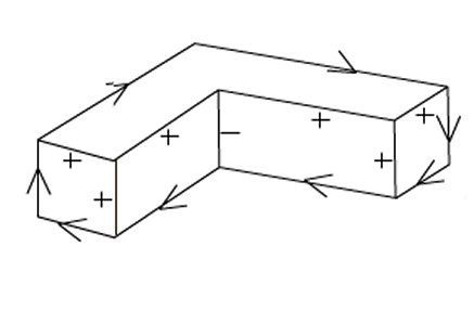
An example of a correctly labelled drawing is given below
How can line-labelling be done automatically? There are some powerful constraints on the possible junction type. These are related to the way surfaces can be arranged in the 3D world. You will deal with this aspect in the (selective) computer vision course. There are four ways of labeling a line, there should be 16 ways of describing an L-junction and 64 ways for each of W,Y and T. So there could be 208 labelled junction types in all. In fact there are only 16 allowed junction types.